BANL 6100: Business Analytics

class: center, middle, inverse, title-slide

.title[
# BANL 6100: Business Analytics
]
.subtitle[
## Analysis of Variance (ANOVA)
]
.author[
### Mehmet Balcilar </br> <a href="mailto:mbalcilar@newhaven.edu" class="email">mbalcilar@newhaven.edu</a>
]
.institute[
### Univeristy of New Haven
]
.date[
### 2024-11-14 (updated: 2024-11-14)
]

---

exclude: true

---
class: center, middle, sydney-blue

<div style = "position:fixed; visibility: hidden">
$$
\require{color}
\definecolor{purple}{rgb}{0.337254901960784, 0.00392156862745098, 0.643137254901961}
\definecolor{navy}{rgb}{0.0509803921568627, 0.23921568627451, 0.337254901960784}
\definecolor{ruby}{rgb}{0.603921568627451, 0.145098039215686, 0.0823529411764706}
\definecolor{alice}{rgb}{0.0627450980392157, 0.470588235294118, 0.584313725490196}
\definecolor{daisy}{rgb}{0.92156862745098, 0.788235294117647, 0.266666666666667}
\definecolor{coral}{rgb}{0.949019607843137, 0.427450980392157, 0.129411764705882}
\definecolor{kelly}{rgb}{0.509803921568627, 0.576470588235294, 0.337254901960784}
\definecolor{jet}{rgb}{0.0745098039215686, 0.0823529411764706, 0.0862745098039216}
\definecolor{asher}{rgb}{0.333333333333333, 0.372549019607843, 0.380392156862745}
\definecolor{slate}{rgb}{0.192156862745098, 0.309803921568627, 0.309803921568627}
\definecolor{cranberry}{rgb}{0.901960784313726, 0.254901960784314, 0.450980392156863}
\definecolor{hi}{rgb}{0.984313725490196, 0.12549019607843137, 0.12549019607843137}
$$
</div>
	
<script type="text/x-mathjax-config">
	MathJax.Hub.Config({
		TeX: {
			Macros: {
				purple: ["{\\color{purple}{#1}}", 1],
				navy: ["{\\color{navy}{#1}}", 1],
				ruby: ["{\\color{ruby}{#1}}", 1],
				alice: ["{\\color{alice}{#1}}", 1],
				daisy: ["{\\color{daisy}{#1}}", 1],
				coral: ["{\\color{coral}{#1}}", 1],
				kelly: ["{\\color{kelly}{#1}}", 1],
				jet: ["{\\color{jet}{#1}}", 1],
				asher: ["{\\color{asher}{#1}}", 1],
				slate: ["{\\color{slate}{#1}}", 1],
				cranberry: ["{\\color{cranberry}{#1}}", 1],
				hi: ["{\\color{hi}{#1}}", 1]
			},
			loader: {load: ['[tex]/color']},
			tex: {packages: {'[+]': ['color']}}
		}
	});
</script>

# Comparing means with ANOVA

---

## Aldrin in the Wolf River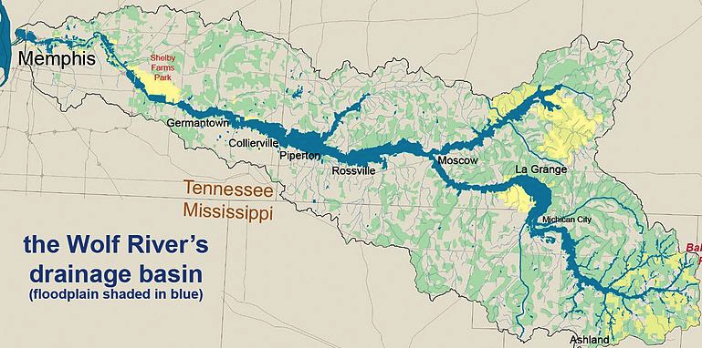

![:scale 50% ](images/lecture12/wolf.png)

- The Wolf River in Tennessee flows past an abandoned site once used by the pesticide industry for dumping wastes, including chlordane (pesticide), aldrin, and dieldrin (both insecticides).
- These highly toxic organic compounds can cause various cancers and birth defects.
- The standard methods to test whether these substances are present in a river is to take samples at six-tenths depth.
- Since these compounds are denser than water and tend to stick to sediment particles, they are more likely to be found in higher concentrations near the bottom.

---

## Data

Aldrin concentration (nanograms per liter) at three levels of depth.

|   | aldrin | depth      |
|---|--------|------------|
| 1 | 3.80   | bottom     |
| 2 | 4.80   | bottom     |
| … | …      | …          |
| 10| 8.80   | bottom     |
| 11| 3.20   | middepth   |
| 12| 3.80   | middepth   |
| … | …      | …          |
| 20| 6.60   | middepth   |
| 21| 3.10   | surface    |
| 22| 3.60   | surface    |
| … | …      | …          |
| 30| 5.20   | surface    |

---

## Exploratory Analysis

Aldrin concentration (nanograms per liter) at three levels of depth.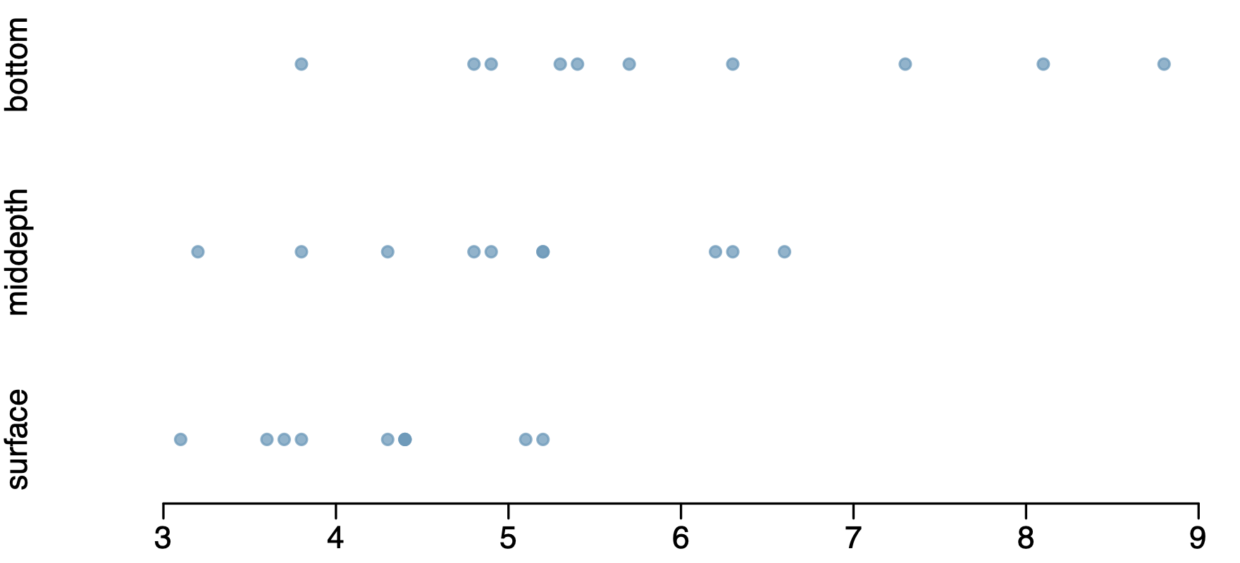

![](images/lecture12/dotplot.png)

|         | n  | mean | sd  |
|---------|----|------|-----|
| bottom  | 10 | 6.04 | 1.58 |
| middepth| 10 | 5.05 | 1.10 |
| surface | 10 | 4.20 | 0.66 |
| overall | 30 | 5.10 | 1.37 |

---

## Research Question

> Is there a difference between the mean aldrin concentrations among the three levels?

- To compare means of 2 groups, use a `$z$` or a Student `$t$` statistic.
- To compare means of 3+ groups, use ANOVA and the `$F$` statistic.

---

## ANOVA

ANOVA assesses whether the mean of the outcome variable is different for levels of a categorical variable.

- **$H_0$:** The mean outcome is the same across all categories,
  $$
  \mu_1 = \mu_2 = \cdots = \mu_k
  $$
  where `$\mu_i$` represents the mean of the outcome for category `$i$`.
- **$H_1$:** At least one mean is different.

- This type of ANOVA is also called One-Way ANOVA, Independent ANOVA, or Between-Subjects ANOVA.

---

## Conditions

1. **Independence**: Observations should be independent within and between groups.
2. **Normality**: Observations within each group should be nearly normal.
3. **Equal Variability**: Variability across the groups should be about equal.

> How do we check for normality?  
> How can we check this condition?

---

## `$z/t$` Test vs. ANOVA - Purpose

### `$z/t$` Test

Compare means from **two** groups to see if they are too far apart to be attributed to sampling variability.
$$
H_0: \mu_1 = \mu_2
$$

### ANOVA

Compare means from **two or more** groups to check if differences can be attributed to sampling variability.
$$
H_0: \mu_1 = \mu_2 = \cdots = \mu_k
$$

---

## `$z$`/$t$ Test vs. ANOVA - Method

### `$z$`/$t$ Test

Compute a test statistic (ratio).
$$
z / t = \frac{(\bar{x}_1 - \bar{x}_2) - (\mu_1 - \mu_2)}{SE(\bar{x}_1 - \bar{x}_2)}
$$

### ANOVA

Compute a test statistic (ratio).
$$
F = \frac{\text{variability between groups}}{\text{variability within groups}}
$$

- Large test statistics lead to small p-values.
- If p-value is small enough, reject `$H_0$`: conclude population means are not equal.

---

## Hypotheses

> What are the correct hypotheses for testing for a difference between the mean aldrin concentrations among the three levels?

1. `$H_0: \mu_B = \mu_M = \mu_S$`, `$H_A: \mu_B \ne \mu_M \ne \mu_S$`
2. `$H_0: \mu_B \ne \mu_M \ne \mu_S$`, `$H_A: \mu_B = \mu_M = \mu_S$`
3. `$H_0: \mu_B = \mu_M = \mu_S$`, `$H_A:$` At least one mean is different.
4. `$H_0: \mu_B = \mu_M = \mu_S = 0$`, `$H_A:$` At least one mean is different.

---

## Test Statistic

> Does there appear to be a lot of variability within groups? How about between groups?

$$
F = \frac{\text{variability between groups}}{\text{variability within groups}}
$$

![](images/lecture12/dotplot_var)

---

## `$F$` Distribution and p-value

$$
F = \frac{\text{variability between groups}}{\text{variability within groups}}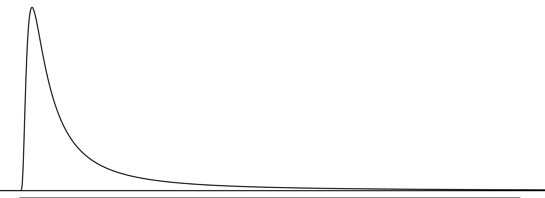
$$

![](images/lecture12/fdist.png)

- A small p-value (large `$F$` statistic) leads to rejecting `$H_0$`.

---

## Conclusion - in Context

> What is the conclusion of the hypothesis test?

The data provide convincing evidence that the average aldrin concentration:

1. Is different for all groups.
2. On the surface is lower than the other levels.
3. **Is different for at least one group.**
4. Is the same for all groups.

---

## Conclusion

- If p-value is small (less than `$\alpha$`), reject `$H_0$`: conclude that at least one mean is different.
- If p-value is large, fail to reject `$H_0$`: conclude differences are due to sampling variability (chance).

---
exclude: true