BANL 6100: Business Analytics

class: center, middle, inverse, title-slide

.title[
# BANL 6100: Business Analytics
]
.subtitle[
## R Notebooks
]
.author[
### Mehmet Balcilar </br> <a href="mailto:mbalcilar@newhaven.edu" class="email">mbalcilar@newhaven.edu</a>
]
.institute[
### Univeristy of New Haven
]
.date[
### 2023-08-28 (updated: 2023-09-25)
]

---

class: center, middle, sydney-blue

# R Notebooks

---

## Getting Work Done

.pull-left[
### Basics of R Notebooks

1. See the [section in R Markdown book](https://bookdown.org/yihui/rmarkdown/notebook.html)
2. See the [description at the RStudio page](https://rmarkdown.rstudio.com/lesson-10.html)
3. [Webinar by Jonathan McPherson](https://resources.rstudio.com/resources/webinars/introducing-notebooks/)
]

.pull-right[
### Notebook Recap

![notebook demo](images/r_notebook/notebook-demo.png)
]

---

## Notebook Recap

- Notebooks are R Markdown documents + new interaction model
- Code chunks are executed individually 
- Code output appears beneath the chunk and is saved with the document 
- Combines iterative approach with reproducible result

If you've never used them before, watch the [R Notebook Webinar](https://www.rstudio.com/resources/webinars/introducing-notebooks-with-r-markdown/)

![webinar](images/r_notebook/webinar.png)

---

## Navigation: Outline

![document outline](images/r_notebook/outline.png)

---

## Navigation: Jump To

![jump to chunk](images/r_notebook/jump-to.png)

---

## Navigation: By Chunk

![prev/next chunk](images/r_notebook/nav-chunks.png)

---

## Navigation: Running

![nav-running](images/r_notebook/nav-running.png)

---

## Output Management

![output-management](images/r_notebook/output-management.png)

---

## Reproducibility

- Notebooks can be **less reproducible** than traditional R Markdown documents.
- Chunks can be run in **any order**. 
- Chunks can access the **global environment**.

## Simulating a Knit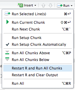

![restart and run](images/r_notebook/restart-and-run.png)

---

## Consistency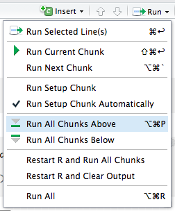

![run chunks above](images/r_notebook/run-chunks-above.png)

---
class: center, middle, sydney-blue

# How R Notebooks *Really* Work

---

## Input and Output

<div class="grViz html-widget html-fill-item-overflow-hidden html-fill-item" id="htmlwidget-f48003c868b2e76ffd7d" style="width:432px;height:504px;"></div>
<script type="application/json" data-for="htmlwidget-f48003c868b2e76ffd7d">{"x":{"diagram":"\ndigraph notebookio {\n  node [shape=\"box\", fontname=\"Helvetica\", fillcolor=lightgrey];\n  doc [label=\"R Markdown (.Rmd)\"];\n  cache [label=\"Local Output Cache\"];\n  edoc [label=\"R Markdown\"];\n  ecache [label=\"Embedded Output Cache\"];\n  rs [label=\"RStudio\"];\n  save [label=\"Save\", shape=\"ellipse\"]\n  execute [label=\"Execute Chunks\", shape=\"ellipse\"]\n  subgraph cluster0 {\n    edoc;\n    ecache;\n    label=\"Notebook HTML (.nb.html)\";\n    labelloc=b;\n  }\n  doc -> save;\n  doc -> execute;\n  cache -> save;\n  save -> edoc;\n  save -> ecache;\n  execute -> cache;\n  doc -> rs;\n  cache -> rs;\n}","config":{"engine":"dot","options":null}},"evals":[],"jsHooks":[]}</script>

---

## Input and Output

1. When you **execute** chunks in your notebook, the output is simultaneously displayed by RStudio and stored in a local cache in the `.Rproj.user` folder.
1. When you **save** your notebook, the output and your R Markdown document are combined into a single, self-contained `.nb.html` file.

---
class: center, middle, sydney-blue

# Publishing and Collaborating

---

## Publishing

Two choices:

1. Publish the notebook file directly (HTML)
1. Render to a separate output format

## Publishing: Notebook HTML

- Self-contained 
- Compatible with any hosting service
- No viewer required
- Hydrates to full notebook (more on this later)

---

## Publishing: Another Format

---
    title: "A Monte-Carlo Analysis of Monte Carlo"
    output:
      html_notebook: default
      pdf_document:
        fig_width: 9
        fig_height: 5
    ---

---

## Understanding Multiple Formats

<div class="grViz html-widget html-fill-item-overflow-hidden html-fill-item" id="htmlwidget-6ca37fc8df4ac4e563ee" style="width:432px;height:504px;"></div>
<script type="application/json" data-for="htmlwidget-6ca37fc8df4ac4e563ee">{"x":{"diagram":"\ndigraph notebookio {\n  node [shape=\"box\", fontname=\"Helvetica\", fillcolor=lightgrey];\n  doc [label=\"R Markdown (.Rmd)\"];\n  cache [label=\"Local Output Cache\"];\n  nb [label=\"Compiled Notebook (.nb.html)\"];\n  pdf [label=\"PDF Publication\"]\n  save [label=\"Save\", shape=\"ellipse\"]\n  execute [label=\"Execute Chunks\", shape=\"ellipse\"]\n  knit [label=\"Knit\", shape=\"ellipse\"]\n  subgraph cluster1 {\n    execute;\n    cache;\n    save;\n    nb;\n    label=\"Develop\";\n  }\n  subgraph cluster2 {\n    knit;\n    pdf;\n    label=\"Present\";\n  }\n  doc -> execute;\n  doc -> knit;\n  knit -> pdf;\n  cache -> save;\n  save -> nb;\n  execute -> cache;\n}","config":{"engine":"dot","options":null}},"evals":[],"jsHooks":[]}</script>

---

## Publishing: RStudio Connect

- One-click publish inside your org
- Fine-grained access control
- Execute on the server
- Schedule executions

## Collaborating: Plain Files

To: analyst@contoso.com
    From: customer@northwind.com
    
    I need some help with this analysis. Could you 
    take a look at what I have so far?
    
    Thanks,
    Charles
    
    [ Attachment: foo.nb.html ]

---

## Collaborating: Execution in Reverse

<div class="grViz html-widget html-fill-item-overflow-hidden html-fill-item" id="htmlwidget-67528883ca73241f749c" style="width:432px;height:504px;"></div>
<script type="application/json" data-for="htmlwidget-67528883ca73241f749c">{"x":{"diagram":"\ndigraph notebookio {\n  compound = true;\n  node [shape=\"box\", fontname=\"Helvetica\", fillcolor=lightgrey];\n  doc [label=\"R Markdown (.Rmd)\"];\n  cache [label=\"Local Output Cache\"];\n  edoc [label=\"R Markdown\"];\n  ecache [label=\"Embedded Output Cache\"];\n  rs [label=\"RStudio\"];\n  open [label=\"Open in RStudio\", shape=\"ellipse\"]\n  view [label=\"View in Browser\", shape=\"ellipse\"]\n  subgraph cluster0 {\n    edoc;\n    ecache;\n    label=\"Notebook HTML (.nb.html)\";\n  }\n  edoc -> open [ltail=cluster0];\n  ecache -> view [ltail=cluster0];\n  doc -> rs;\n  cache -> rs;\n  open -> doc;\n  open -> cache;\n}","config":{"engine":"dot","options":null}},"evals":[],"jsHooks":[]}</script>

---

## Collaborating: Opening Code in RStudio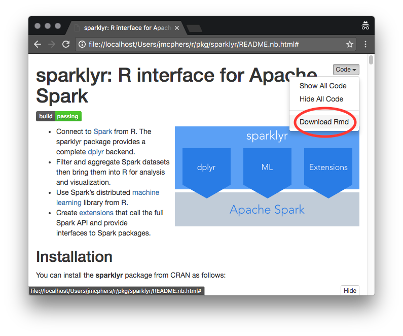

![download R markdown](images/r_notebook/download-rmd.png)

---

## Collaborating: Opening Notebook in RStudio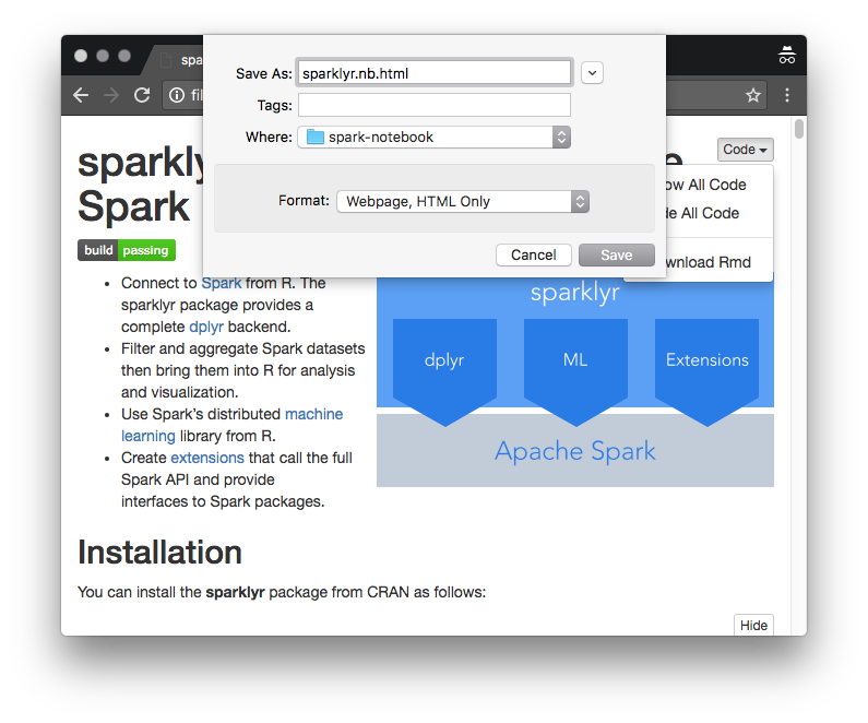

![save as notebook](images/r_notebook/save-as-nb-html.png)

---

## Collaborating: Open Inside RStudio

![pre open](images/r_notebook/pre-open.png)

---

## Collaborating: Open Notebook

![hydrated](images/r_notebook/hydrated-notebook.png)

---

## Collaborating: Version Control #1

- Add `*.nb.html` to your `.gitignore` or similar
- Check in only the `.Rmd` file
- All diffs are plain text
- Encourages reproducibility & independent verification of results

## Collaborating: Version Control #2

- Check in the `.nb.html` file and the `.Rmd` file
- Diffs are noisier
- RStudio loads outputs from `.nb.html` if newer
- Outputs and inputs are versioned together
- No need to re-execute lengthy or fragile computations

---

## Versioned Output

When a notebook is opened:

- The local cache modified time is compared to the `.nb.html` 
- If `.nb.html` is older, it is ignored
- If `.nb.html` is newer, it replaces the local cache
- No merging or conflict management is performed!

---

## The End

![:scale 50%](images/r_notebook/lego-cat.jpg)